Logistic Regression

The simple answer is the logistic regression is a way to classify a binary target. So if you have a bunch of features in order to tell you if you’re looking at a dog or a cat, you could in theory train a logistic regression algorithm on said features to tell you the next time you see an animal if the animal is a dog or a cat.

The slightly more in depth answer is that the logistic equation is defined like so:

\[ p(\bar{X}) = \dfrac{e^{\beta_{0} + \beta_{1}X_{1} + \dots + \beta_{p}X_{p}}}{1 + e^{\beta_{0} + \beta_{1}X_{1} + \dots + \beta_{p}X_{p}}} \]

Where we have \(p(\bar{X})\) being the “real” function that defines the relationship between the features encoded in \(\bar{X} = (X_{0}, X_{1}, \dots , X_{p})\), and the coefficients \(\beta_{0}, \dots , \beta_{p}\) are the coefficients which are “learned” in the machine learning process.

Now any good statistics teacher will tell you that his isn’t the extent of what you should learn about logistic regression. However, I’m no statistics teacher (nor do I currently have time to go through this), so what I’ll say is that if you’re reading this post you should also take a look at the book Introduction to Statistical Learning which has a great discussion on this topic in Chapter 4. I’d also recommend this for anyone at all trying to learn statistics.

Great! Moving forward bravely to the next step, we’re going to look at how to use this for a very contrived and annoying problem, which we’re going to not only create ourselves, but we’ll also solve ourselves. Why? Because that’s the best way to learn, change my mind. So the basic idea is that we want to have certain features which will create a relatively binary output. We also want the target to rely on the features, in a binary fashion. That’s simple enough:

Data Generation

Code

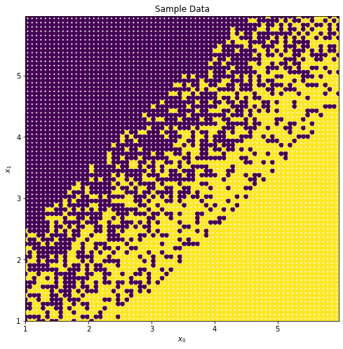
import numpy as np
import matplotlib.pyplot as plt


def make_sample_data(minimum, maximum, resolution=1):
    """
    Creates a grid of data points with a rough boundary line separating them in 2D.

    Basic rule is:
    x - y + noise >= -0.5

    Args:
        minimum      (int): Start point
        maximum      (int): End point
        resolution (float): How closely you want the points to be packed

    Returns:
        xx     (np.array): x coordinates
        yy     (np.array): y coordinates
        target (np.array): 1/0 output array based on rule
    """
    x1 = np.arange(minimum, maximum, resolution)
    x2 = np.arange(minimum, maximum, resolution)
    xx, yy = np.meshgrid(x1, x2)
    target = 10 * (
        xx - yy + np.random.randint(low=-2, high=2, size=(len(xx), len(yy))) >= -0.5
    )
    return xx, yy, target


x_sample, y_sample, target_sample = make_sample_data(1, 6, resolution=0.07)

plt.figure(figsize=(8, 8))
plt.title("Sample Data")
plt.scatter(x_sample, y_sample, c=target_sample)
plt.xlim(left=min(x_sample[0]), right=max(x_sample[0]))
plt.ylim(bottom=min(x_sample[0]), top=max(x_sample[0]))
plt.xlabel(r"$x_{0}$")
plt.ylabel(r"$x_{1}$")
plt.show()

Taking a look at the data we’ve created, we can say that there’s a (relatively) clear boundary present. The rule that I implemented is:

\[ f(\bar{X}) = \begin{cases} 1, & x_{0} - x_{1} + \epsilon \geq -0.5 \\ 0, & \text{otherwise} \end{cases} \]

Where \(\bar{X} = (x_{0}, x_{1})\)

So in the case of \(\bar{X} = (2, 4)\) we have that the output will be -2, making the value of our function 1. That looks to chek out when we look at our figure above.

Model Building

Now on to the part that most of you are here for: building a logistic model using sklearn

Code

from sklearn.linear_model import LogisticRegression
import pandas as pd

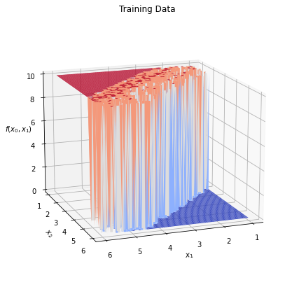
One last time, let’s take a look at our data, but in a different way this time. Lets look at it in 3D, so we can see the literal sigmoidal nature of our model:

Code

fig = plt.figure(figsize=(14, 7))
ax = plt.axes(projection="3d")
ax.plot_surface(
    x_sample, y_sample, target_sample, cmap="coolwarm", rcount=200, ccount=200
)
ax.set_xlabel(r"$x_1$")
ax.set_ylabel(r"$x_2$")
ax.zaxis.set_rotate_label(False)
ax.set_zlabel(r"$f(x_{0},x_{1})$", rotation=0)
ax.view_init(15, 70)
plt.title("Training Data")
plt.show()

Note the little section in the middle where we’ve added uncertainty. Everything else is relatively concrete in the output (we’re keeping it simple).

Next step that we want to put our data in a nice dataframe and use LogisticRegression from sklearn.linear_model. This has some default that we’re going to use. Specifically, the “penalty” assigned to our training is the L2 norm. I’m going to make a post about the different types of penalty, but let’s keep it moving for now.

df = pd.DataFrame(
    {"x1": x_sample.ravel(), "x2": y_sample.ravel(), "target": target_sample.ravel()}
)

df.head()

	x1	x2	target
0	1.00	1.0	0
1	1.07	1.0	10
2	1.14	1.0	10
3	1.21	1.0	0
4	1.28	1.0	0

There’s our little table, and here’s how we can fit the logistic regression with the defaults:

model = LogisticRegression(random_state=0)
model.fit(df[["x1", "x2"]], df.target)

LogisticRegression(random_state=0)

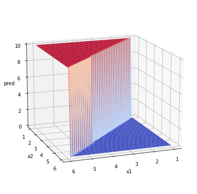
Now that we’ve fitted our data, we can do a few things. Yes, we can predict, but also importantly we can learn about the model itself. Remember the basic structure of the model? Well now we can determine what our model should have looked like. There are a few ways we can go about this, namely we can use the model.coef_ and model.intercept to manually calculate the output values, or we can just use model.predict. Now keep in mind I’m running the prediction on the training data, mainly so I can see if the structure was captured:

Code

df["predictions"] = model.predict(df[["x1", "x2"]])
fig = plt.figure(figsize=(14, 7))
ax = plt.axes(projection="3d")
ax.plot_surface(
    x_sample, y_sample, df[["predictions"]].to_numpy().reshape(72, 72), cmap="coolwarm"
)
ax.set_xlabel("x1")
ax.set_ylabel("x2")
ax.set_zlabel("pred")
ax.view_init(15, 70)
plt.show()

That looks extremely similiar to the idea we had when we created the data. So on that note, I’m going to leave the basics of logistic regression here. Next up we can take a closer look at prediction and accuracy of the model.