Alright, so this is going to be a quick, not very in depth approach to linear regression with TensorFlow. A lot of the functions I’m using for this that have to do with TensorFlow will be explained in a later post where I describe everything as simply as possible with examples. Bear with me here. One note is that I’m taking section 3.2 of the d2l.ai book and trying to make it simpler, so you may see code overlap, but hopefully this will be much more informative and easier to read (after some revisions).
Data Generation
The simplest way to start as I always to is to generate the data. In this case, we’re looking to generate the data which has two features and one output. So our true equation will be of the form: \[ y = \underline{X}\bar{w} + \bar{b} \] Where \(\underline{X}\) is a matrix, \(\bar{w}, \bar{b}\) are vectors. It’s important to know the dimensions of our matrix and vectors. Here we have \(\underline{X}\) in the shape of (num_samples, num_features). So really that should be (\(n\), 2) where \(n\) is the number of samples we have. Our vectors on the other hand will be of the shape:
- \(w\): (num_samples, 1)
- \(b\): (num_samples, 1)
To be as clear as possible, our equation looks like this:
\[ \begin{bmatrix} y_1 \\ \vdots \\ y_n \end{bmatrix} = \begin{bmatrix} x_{1,1} & x_{1,2} & \dots & x_{1, p} \\ x_{2,1} & x_{2,2} & \dots & x_{2, p} \\ \vdots & & \ddots & \vdots \\ x_{n, 1} & x_{n, 2} & \dots & x_{n, p} \end{bmatrix} \begin{bmatrix} w_1 \\ \vdots \\ w_p \end{bmatrix} + \begin{bmatrix} b_1 \\ \vdots \\ b_n \end{bmatrix} \]
By the way… this isn’t how you should usually look at linear regression. Usually you’d include \(\bar{b}\) in \(\underline{X}\) and \(\bar{w}\), but to be more clear we’ll seperate it here.
Last thing to keep in mind is that we’re adding noise (because otherwise it’s not very fun!). That noise vector \(\bar{\epsilon}\) will also have a shape of (\(n\), 1), making our final equation:
\[ \begin{bmatrix} y_1 \\ \vdots \\ y_n \end{bmatrix} = \begin{bmatrix} x_{1,1} & x_{1,2} & \dots & x_{1, p} \\ x_{2,1} & x_{2,2} & \dots & x_{2, p} \\ \vdots & & \ddots & \vdots \\ x_{n, 1} & x_{n, 2} & \dots & x_{n, p} \end{bmatrix} \begin{bmatrix} w_1 \\ \vdots \\ w_p \end{bmatrix} + \begin{bmatrix} b_1 \\ \vdots \\ b_n \end{bmatrix} + \begin{bmatrix} \epsilon_1 \\ \vdots \\ \epsilon_n \end{bmatrix} \]
def generate_data(w, b, num_samples):
    """
    Create sample data of the form

    y = Xw + b + epsilon

    Where epsilon is random noise centered around 0, std dev 0.01
    """
    X = tf.random.normal(shape=(num_samples, w.shape[0]))
    w_reshaped = tf.reshape(w, shape=(-1, 1))
    epsilon = tf.random.normal(shape=(num_samples, 1), stddev=0.01)
    y = tf.matmul(X, w_reshaped) + b + epsilon
    return X, y


true_w = tf.constant([2, -3.4])
true_b = 4.2

features, labels = generate_data(true_w, true_b, 1000)
Data Visualization
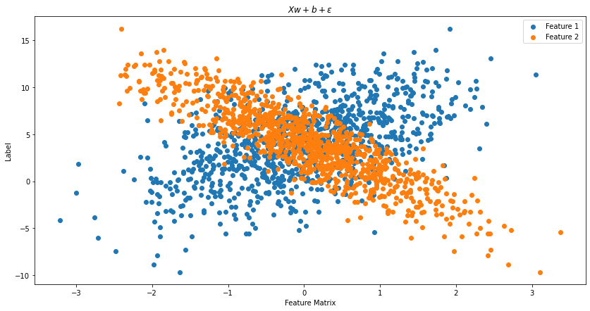
Now we used simple parameters of \(w_1 = 2\) and \(w_2 = -3.4\), with \(b = 4.2\). Here’s what our features look like:
Code
Code
fig = plt.figure(figsize = (14,14))
ax = plt.axes(projection='3d')
ax.scatter3D(features[:, 0],
             features[:, 1],
             labels, cmap = 'coolwarm')
ax.set_xlabel(r"$x_1$")
ax.set_ylabel(r"$x_2$")
ax.zaxis.set_rotate_label(False)
ax.set_zlabel(r"$y$", rotation = 0)
ax.view_init(20, 140)
plt.title("Training Data")
plt.show()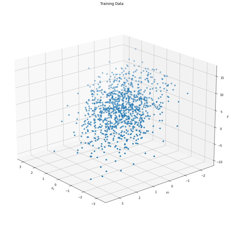
As our second feature \(X_{n, 2}\) gets more negative and our first feature \(X_{n, 1}\) gets more positive, we see that the response variable \(y\) increases. We can clearly see the relationship between our features, so let’s see now if our model can as well!
Training & (minibatch stochiastic) Gradient Descent
This section is going to cover a few things. Specifically
- What the hell is gradient descent?
- Why do we batch things (also what does it mean to batch things)?
- Why are we using minibatch and what the hell is it anyway?
Gradient Descent
Gradient descent is an optimization algorithm. The main point of it is to find the minimum or maximum of a particular surface which is defined by a differentiable function. The obvious question to the layman at this point is going to be: what the hell do any of those words mean Darpan? Fair enough. Let’s get some examples going.
A simple example of a “differentiable” function is the function \(f(x) = x^2\). Why is it differentiable? Because you can find the effect that changing the input will have on the out for all points (technically all points in the functions domain). That’s pretty much it. Here’s what I mean:
\[ \dfrac{d}{dx} (x^2) = 2x \]
Why does that matter? Because gradient descent is an algorithm which looks at the fact that when you take the derivative of a given function (lets call that \(f'(x)\)) and plug in values, you can see how steep the original function is. Let me show you what I mean:
x = np.linspace(-10, 10)
f = x**2

plt.figure(figsize = (14,7))
plt.title("Derivative")
plt.xlim(left = min(x), right = max(x))
plt.ylim(-40, 100)
plt.plot(x, f, label = 'Original Function')
plt.plot(x, [4*i - 4 for i in x], label = 'Rate of change at x = 2')
plt.vlines(x = 2, ymin = -40, ymax = 100, linestyles='--', color='red')
plt.legend()
plt.show()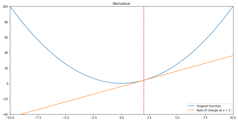
We see above that the steepness can be measured via finding the derivative of our original function at the point of x = 2:
\[ \begin{aligned} f'(x = 2) &= \dfrac{d}{dx}(x^2) \\ &= 2x \\ &= 2(2) \\ f'(x = 2) &= 4 \end{aligned} \]
And that’s exactly the slope of the orange line! Similarly, if we look at when \(x = 5\), we end up with \(f'(x) = 2(5) = 10\). That means the slope is higher on the edges of the domain (our \(x\) values), and lower toward the center (\(x = 0\)). Turns out the center is exactly where our function’s minimum value is!
Now if we imagine we’re starting at \(x = 5\) and trying to get to the lowest possible value of our function, we know we have to go toward 0. Why is it that we know this? Because our brains are processing the shape and seeing “hey that’s where we’re getting the lowest.”
The (naive) way to get a computer to see this is through gradient descent. Here’s the general idea in mathematical form:
\[ a_{n+1} = a_{n} - \gamma \nabla F(a_n) \]
So the entire thing above says “I’m gonna measure the slope where I’m at, and go toward the place which has the steepest slope downward.” That’s it, seriously.
- \(a_n\) is our current location (e.g. \(x = 5\))
- \(\gamma\) is how large our steps are (e.g. should we go from 5 to 5.1 or from 5 to 5.01?)
- \(\nabla F(a_n)\) is the gradient (a derivative in multiple dimensions) at the place we’re at (trying to figure out which way is an increasing slope and which way is a decreasing slope)
In our case, the slope would be the error or loss between the predicted function and the actual values.
There is a lot more to say about how exactly this works and why it matters so much, but this has already been more than a bite sized post so I’ll leave it at that.
Batches ’n Stuff
There is a small but great article here which explains it more thoroughly than I will at the moment.
Essentially batches are subsets of the dataset which you feed into the training loop. After one batch has been fed into the training loop, you use the results to update your model parameters. So if you have a dataset of size 100, you may take a batch size of 20, which would mean for each epoch, you’d have to update your parameters 5 times. You can refer to this as minibatch gradient descent. We’ll be using a batch size of 10. Given that our dataset has the size of 1,000 we know the number of times the parameters are updated in one epoch is:
\[ \dfrac{\text{Dataset Size}}{\text{Batch Size}} = \dfrac{1000}{10} = 100 \text{ times} \]
def data_iter(batch_size, features, labels):
    """
    Creating minibatches to use in training
    """
    num_examples = len(features)
    indicies = list(range(num_examples))
    random.shuffle(indicies)
    for i in range(0, num_examples, batch_size):
        j = tf.constant(indicies[i : min(i + batch_size, num_examples)])
        yield tf.gather(features, j), tf.gather(labels, j)
The rest of the code here should be relatively clear, but if it isnt here’s a brief summary:
linear_regression: Performs the actual linear regression with the tensorflow functionmatmulsquared_loss: Calculates the squared loss between the predicted and the actual values (MSE)
The final training loop simply takes the values of the number of epochs (i.e. the number of times we want to complete a training iteration) and applies the tensorflow implementation of gradient to our function, with respect to our losses and the current weights and biases. Take some time to play with this if you aren’t clear (and print things out!).
def linear_regression(X, w, b):
    return tf.matmul(X, w) + b

def squared_loss(y_hat, y):
    return (y_hat - tf.reshape(y, y_hat.shape))**2 / 2

def sgd(params, grads, lr, batch_size):
    for param, grad in zip(params, grads):
        param.assign_sub(lr*grad/batch_size)

w = tf.Variable(tf.random.normal(shape=(2, 1), mean=0, stddev=0.01),
                trainable=True)
b = tf.Variable(tf.zeros(1), trainable=True)

lr = 0.03
num_epochs = 3
net = linear_regression
loss = squared_loss


for epoch in range(num_epochs):
    for X, y in data_iter(batch_size=10, features=features, labels=labels):
        with tf.GradientTape() as g:
            l = loss(net(X, w, b), y)
        dw, db = g.gradient(l, [w, b])
        sgd([w, b], [dw, db], lr, batch_size=10)
    train_l = loss(net(features, w, b), labels)
    print(f"Epoch {epoch+1}, loss {float(tf.reduce_mean(train_l)):f}")
This is an abrupt stop, because I’ve got yet another thing I’d like to obsess about. Coming soon!